2. Small Worlds and Large Worlds

Example (p. 33)

The likelihood of the data: 6 W in 9 tosses, under the probability of 0.5

dbinom(6, size=9, prob=0.5)

[1] 0.1640625

Grid Approximation

For the globe tossing example, let’s make a grid of 20 points

# change this for more precision. however, there will not be much change in inference after 100 points
num_of_points = 20

# 1. define grid
p_grid <- seq(from=0, to=1, length.out=num_of_points)

# 2. define prior
prior <- rep(1, num_of_points)

# 3. compute likelihood at each value in the grid
likelihood <- dbinom(6, size=9, prob=p_grid)

# 4. compute product of likelihood and prior
unstd.posterior <- likelihood * prior

# 5. standarize the posterior, so it sums to 1
posterior <- unstd.posterior / sum(unstd.posterior)

Let’s display the posterior distribution:

plot(p_grid, posterior, type="b", xlab = "prob. of water", ylab="posterior prob.")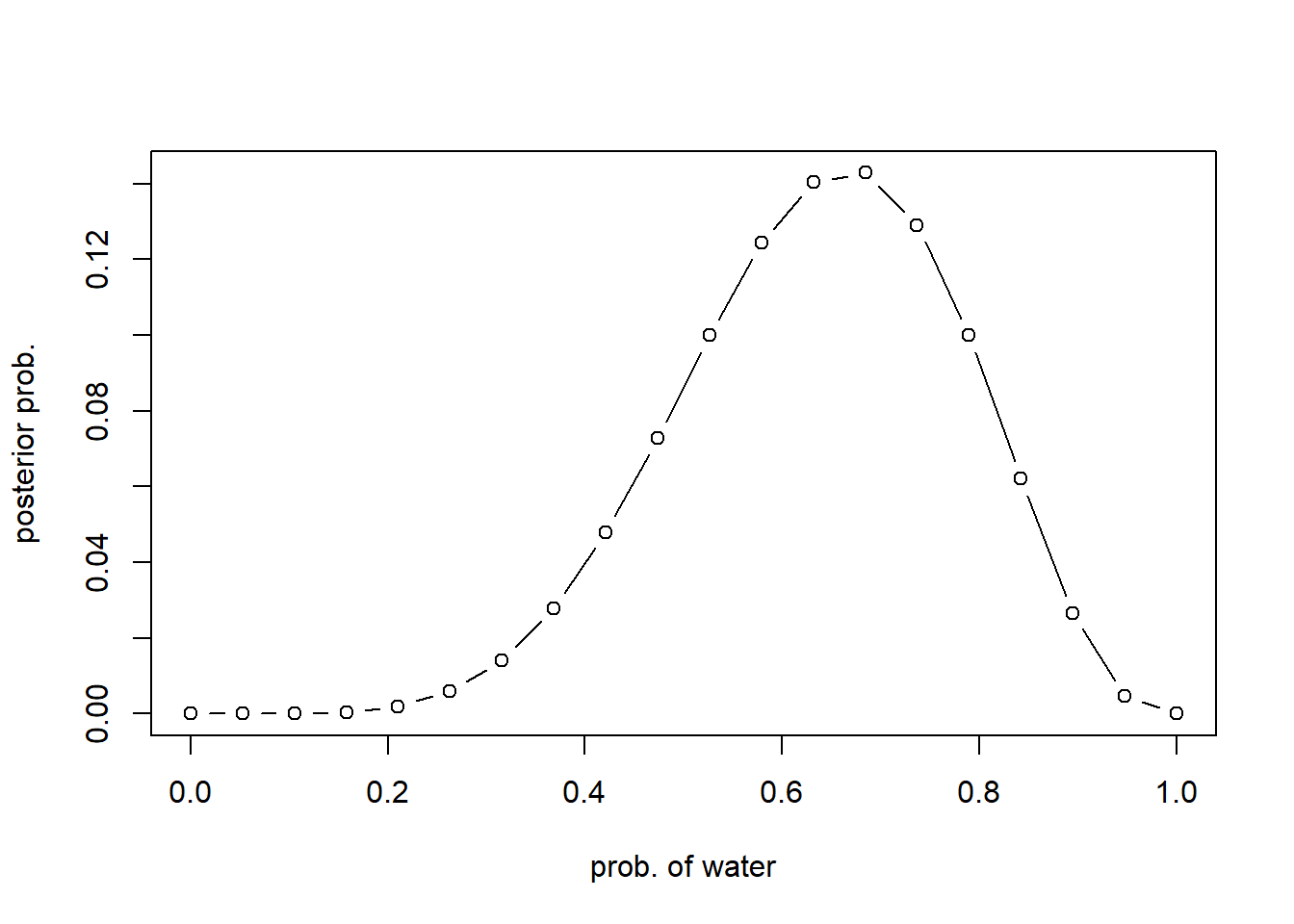

Different prior #1:

num_of_points = 20

# 1. define grid
p_grid <- seq(from=0, to=1, length.out=num_of_points)

# 2. define prior
prior <- ifelse(p_grid < 0.5, 0, 1)

# 3. compute likelihood at each value in the grid
likelihood <- dbinom(6, size=9, prob=p_grid)

# 4. compute product of likelihood and prior
unstd.posterior <- likelihood * prior

# 5. standarize the posterior, so it sums to 1
posterior <- unstd.posterior / sum(unstd.posterior)

# 6. plot
plot(p_grid, posterior, type="b", xlab = "prob. of water", ylab="posterior prob.")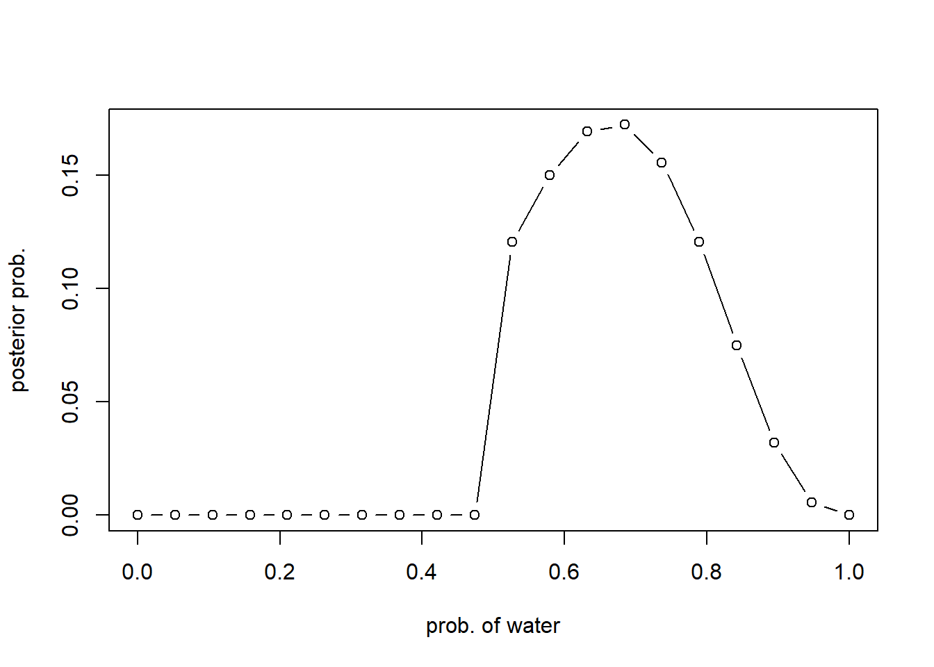

Different prior #2:

num_of_points = 20

# 1. define grid
p_grid <- seq(from=0, to=1, length.out=num_of_points)

# 2. define prior
prior <- exp(-5*abs(p_grid - 0.5))

# 3. compute likelihood at each value in the grid
likelihood <- dbinom(6, size=9, prob=p_grid)

# 4. compute product of likelihood and prior
unstd.posterior <- likelihood * prior

# 5. standarize the posterior, so it sums to 1
posterior <- unstd.posterior / sum(unstd.posterior)

# 6. plot
plot(p_grid, posterior, type="b", xlab = "prob. of water", ylab="posterior prob.")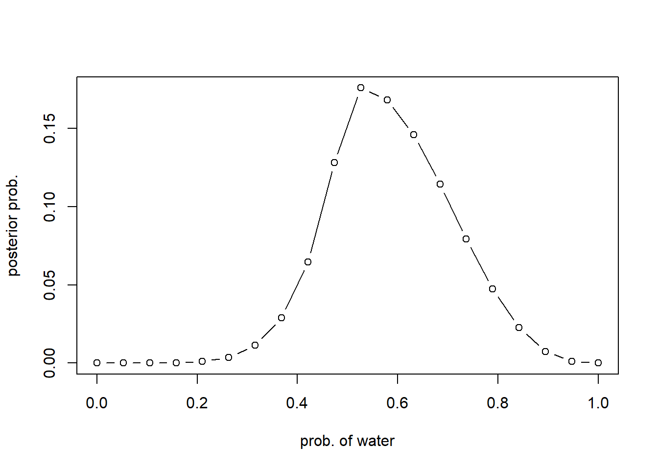

Quadratic Approximation

a.k.a. Gaussian Approximation, because we assume that the posterior is Gaussian

library(rethinking)

Loading required package: cmdstanr

This is cmdstanr version 0.7.1

- CmdStanR documentation and vignettes: mc-stan.org/cmdstanr

- CmdStan path: C:/Users/H/Documents/.cmdstan/cmdstan-2.34.1

- CmdStan version: 2.34.1


A newer version of CmdStan is available. See ?install_cmdstan() to install it.
To disable this check set option or environment variable CMDSTANR_NO_VER_CHECK=TRUE.

Loading required package: posterior

This is posterior version 1.5.0


Attaching package: 'posterior'

The following objects are masked from 'package:stats':

    mad, sd, var

The following objects are masked from 'package:base':

    %in%, match

Loading required package: parallel

rethinking (Version 2.40)


Attaching package: 'rethinking'

The following object is masked from 'package:stats':

    rstudent

globe.qa <- quap(
  
  alist(
    W ~ dbinom(W+L, p),  # binomial likelihood
    p ~ dunif(0, 1)     # uniform prior
  ),
  
  data=list(W=6, L=3)
  
)

# print a summary of quadratic approx.
precis(globe.qa)

       mean        sd      5.5%     94.5%
p 0.6666667 0.1571338 0.4155366 0.9177968

The output refers to the properties of the posterior, assuming it is Gaussian. Let’s compare this approximation with the real posterior distribution (it has a Beta distribution analytically)

W <- 6
L <- 3

# from the previous outputs
globe.qa.mean <- 0.67
globe.qa.sd <- 0.16

# the real posterior distribution
curve(dbeta(x, W+1, L+1), from=0, to=1)

# the quadratic/gaussian approximation
curve(dnorm(x, globe.qa.mean, globe.qa.sd), lty=2, add=TRUE)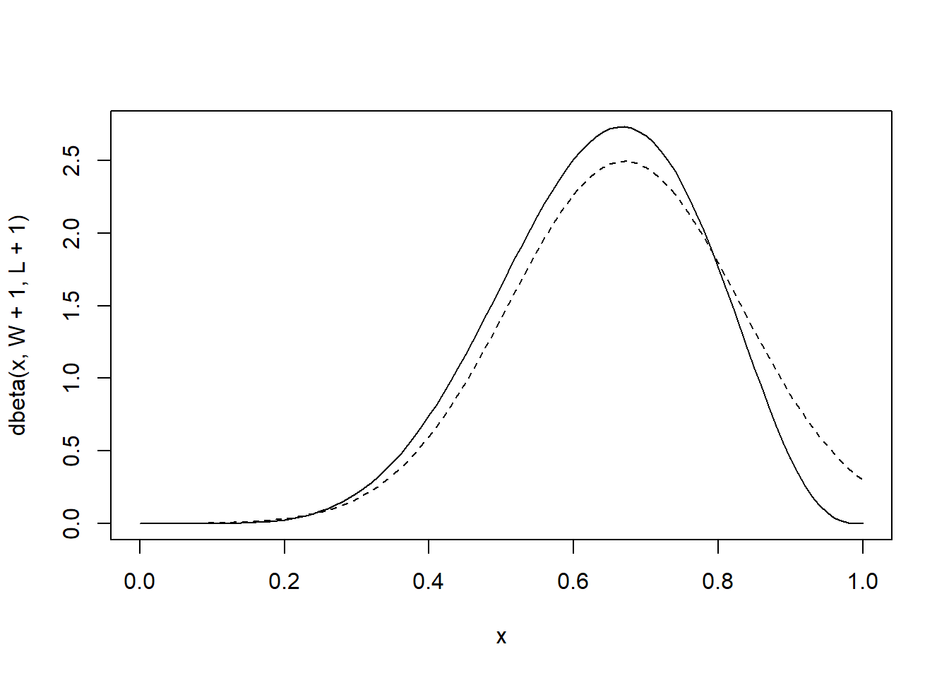

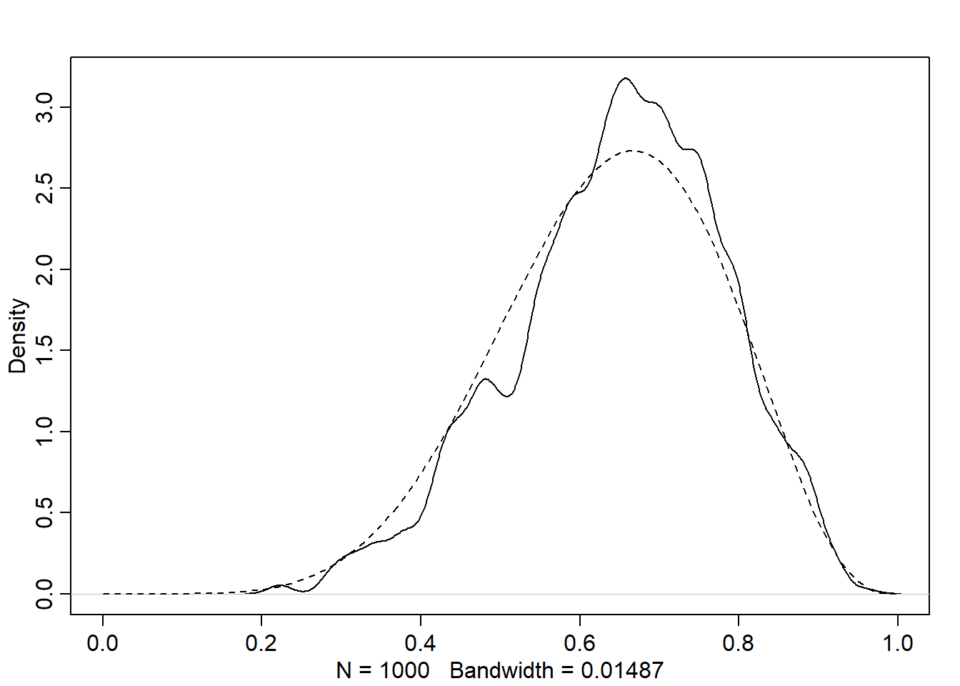
Markov Chain Monte Carlo (MCMC)

n_samples <- 1000
p <- rep(NA, n_samples)
p[1] <- 0.5

W <- 6
L <- 3

for (i in 2:n_samples) {
  p_new <- rnorm(1, p[i-1], 0.1)
  if (p_new < 0) p_new <- ans(p_new)
  if (p_new > 1) p_new <- 2 - p_new
  q0 <- dbinom(W, W+L, p[i-1])
  q1 <- dbinom(W, W+L, p_new)
  p[i] <- ifelse(runif(1) < q1/q0, p_new, p[i-1])
}

# compare the MCMC approximation with the analytical posterior (beta) 
dens(p, xlim=c(0,1))
curve(dbeta(x, W+1, L+1), lty=2, add=TRUE)