5. The Many Variablles and The Spurious Waffles

The dataset WaffleDivorce contains data om divorce rate, marraige rate, and median marriage age.

Let’s load the data first

library(rethinking)

Loading required package: cmdstanr

This is cmdstanr version 0.7.1

- CmdStanR documentation and vignettes: mc-stan.org/cmdstanr

- CmdStan path: C:/Users/H/Documents/.cmdstan/cmdstan-2.34.1

- CmdStan version: 2.34.1

Loading required package: posterior

This is posterior version 1.5.0


Attaching package: 'posterior'

The following objects are masked from 'package:stats':

    mad, sd, var

The following objects are masked from 'package:base':

    %in%, match

Loading required package: parallel

rethinking (Version 2.40)


Attaching package: 'rethinking'

The following object is masked from 'package:stats':

    rstudent

data("WaffleDivorce")
d <- WaffleDivorce

Let’s explore the associations:

Divorce rate with median age at marriage

plot(Divorce~MedianAgeMarriage, data=d, xlim=c(20,30), ylim=c(5,20))

Divorce rate with marriage rate

plot(Divorce~Marriage, data=d, xlim=c(10,30), ylim=c(5,20))

It looks like the associations are reversed.

Model 1: D ~ A

Here’s the model linear regression model for the 1st association: \[ D_i \sim N(\mu_i, \sigma) \] \[ \mu_i = \sigma + \beta_A A_i \]

\[ \alpha \sim N(0, 0.2) \]

\[ \beta \sim N(0, 0.5) \]

\[ \sigma \sim Exp(0, 0.5) \]

Before coding the model, let’s standardize variables.

# standardize variables
d$D <- standardize(d$Divorce)
d$M <- standardize(d$Marriage)
d$A <- standardize(d$MedianAgeMarriage)

By standardizing the variables, we can say that if \(\beta_A=1\), then a change of 1 std. deviation in \(A_i\) is associated with a full std. deviation change in the outcome variable.

m5.1 <- quap(
  alist(
    D ~ dnorm(mu, sigma),
    mu <- a+bA*A,
    a ~ dnorm(0, 0.2),
    bA <- dnorm(0, 0.5),
    sigma ~ dexp(1)
  ),
  data=d
)

set.seed(10)
prior <- extract.prior(m5.1)
mu <- link(m5.1, post=prior, data=list(A=c(-2,2)))
plot(NULL, xlim=c(-2,2), ylim=c(-2,2))
for(i in 1:50) lines(c(-2,2), mu[i,], col=col.alpha("black", 0.4))

A_seq <- seq(-3,3.2,30)
mu <- link(m5.1, data=list(A=A_seq))
mu.mean <- apply(mu, 2, mean)
mu.PI <- apply(mu, 2, PI, prob=0.89)

{
  plot(D~A, data=d, col=rangi2)
  lines(A_seq, mu.mean, lwd=2)
  shade(mu.PI, A_seq)
}

Model 2: D ~ M

\[ D_i \sim N(\mu_i, \sigma) \] \[ \mu_i = \sigma + \beta_M M_i \]

\[ \alpha \sim N(0, 0.2) \]

\[ \beta_M \sim N(0, 0.5) \]

\[ \sigma \sim Exp(0, 0.5) \]

m5.2 <- quap(
  alist(
    D ~ dnorm(mu, sigma),
    mu <- a+bM*A,
    a ~ dnorm(0, 0.2),
    bM <- dnorm(0, 0.5),
    sigma ~ dexp(1)
  ),
  data=d
)

DAGs

Let’s assume the possible causal models that are connected to the divorce rate association examples

Proposed DAG Model 1

library(dagitty)
DMA1 <- dagitty('dag{D <- A -> M -> D}')
drawdag(DMA1)

impliedConditionalIndependencies(DMA1)
# no output because there is no conditional independence

Proposed DAG Model 2

DMA2 <- dagitty('dag{D <- A -> M}')
drawdag(DMA2)

impliedConditionalIndependencies(DMA2)

D _||_ M | A

Model 3: Multiple Regression

\[ D_i \sim N(\mu_i, \sigma) \] \[ \mu_i = \sigma + \beta_M M_i + \beta_A A_i \]

\[ \alpha \sim N(0, 0.2) \]

\[ \beta_M \sim N(0, 0.5) \] \[ \beta_A \sim N(0, 0.5) \]

\[ \sigma \sim Exp(0, 0.5) \]

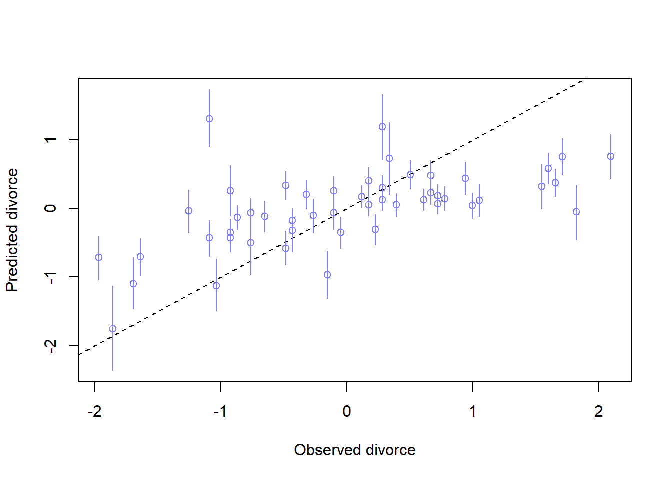
m5.3 <- quap(
  alist(
    D ~ dnorm(mu, sigma),
    mu <- a + bM*M + bA*A ,
    a ~ dnorm(0, 0.2),
    bA <- dnorm(0, 0.5),
    bM <- dnorm(0, 0.5),
    sigma ~ dexp(1)
  ),
  data=d
)
precis(m5.3)

               mean         sd       5.5%      94.5%
a     -4.383618e-05 0.09707212 -0.1551838  0.1550962
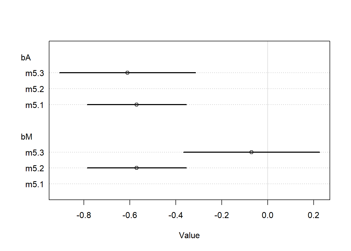
bA    -6.134983e-01 0.15097697 -0.8547887 -0.3722079
bM    -6.546454e-02 0.15076527 -0.3064166  0.1754875
sigma  7.850766e-01 0.07783322  0.6606841  0.9094691

plot(coeftab(m5.1,m5.2,m5.3), par=c("bA", "bM"))

We can read this result as: > Once we know median age at marriage for a state, there is little or no additional predictive power in also knowing the rate of marriage in that state.

Intuitive explanation: The plot shows that the coefficient for the median age at marriage (bA) is quite stable across models (m5.1 and m5.3), while the coefficient for the marriage rate (bM) is less stable and moves towards zero when both predictors are included. This indicates that the median age at marriage is capturing most of the variability that the marriage rate would also explain. Thus, once you know the median age at marriage, the marriage rate doesn’t add much new information (predictive power) for the outcome of interest.

Results: - DAG 1 implies this result. - The association between marriage rate \(M\) and \(D\) divorce rate is spurious and caused by the influence of age of marriage on both \(M\) and \(D\). - Strictly speaking: \(D \amalg M|A\)

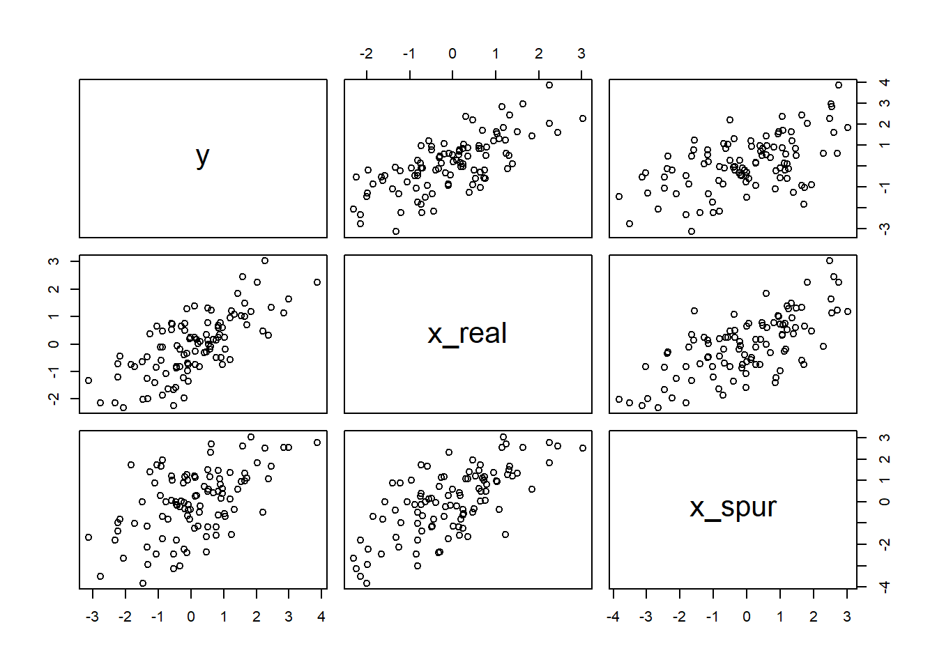
Simulating spurious association

Let’s simulate the association in the DAG:

N <- 100
x_real <- rnorm(N)
x_spur <- rnorm(N, x_real)
y <- rnorm(N, x_real)
d <- data.frame(y, x_real, x_spur)
pairs(d)

Plotting multivariate posterior

The book covered 3 kinds of plots:

1. Predictor residual

Predictor residual is the average prediction error when we use all of the other predictor variables to model a predictor of interest

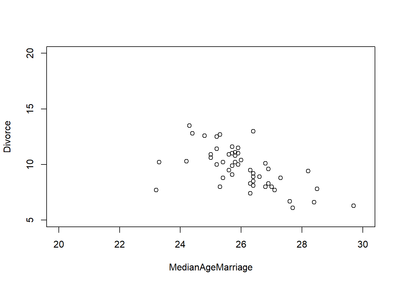
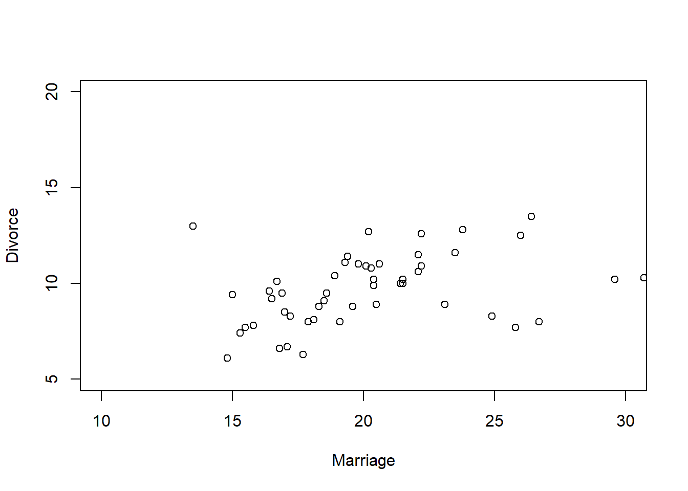
data("WaffleDivorce")
d <- WaffleDivorce

d$D <- standardize(d$Divorce)
d$M <- standardize(d$Marriage)
d$A <- standardize(d$MedianAgeMarriage)

m5.4 <- quap(
  alist(
    M ~ dnorm(mu, sigma),
    mu <- a + bAM * A, 
    a ~ dnorm(0, 0.2),
    bAM ~ dnorm(0, 0.5),
    sigma ~ dexp(1)
  ), data=d
)

mu <- link(m5.4)
mu_mean <- apply(mu, 2, mean)
mu_resid <- d$M - mu_mean

2. Posterior prediction plots

mu <- link(m5.3)
mu_mean <- apply(mu, 2, mean)
mu_PI <- apply(mu, 2, PI)

D_sim <- sim(m5.3, n=1e4)
D_PI <- apply(D_sim, 2, PI)

{
  plot(mu_mean ~ d$D, col=rangi2, ylim=range(mu_PI),
       xlab="Observed divorce", ylab="Predicted divorce")
  
  abline(a=0, b=1, lty=2)
  for(i in 1:nrow(d)) lines(rep(d$D[i], 2), mu_PI[,i], col=rangi2)

}

3. Counterfactual plots

This displays the causal implications of the model. They help you understand the model, as well as generate predictions for imaginary interventions and compute how much some observed outcome could be attributed to some cause.

The basic recipe: 1. Set the assumed scientific model (e.g. draw the DAG) 2. Pick the intervention variable (i.e. variable to manipulate) 3. Define the range of values to set the intervention variable to 4. Do the following simulation:

For each value of intervention variable:
  For each sample in posterior:
    Use the causal model to simulate the values of other variables including the outcome

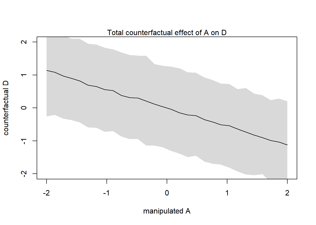
DAG Model 1

For the divorce model (represented by the DAG 1), we need a set of functions that tell us how each variable is generated. We will follow the same approach we did in the m5.3 but with adding the influence of A on M, since in the previous models we cared about estimating A -> D influence. Now, we need to predict the consequences of manipulating A. Estimating the influence of A on M is conducting by regressing A on M.

d <- list()
d$A <- standardize(WaffleDivorce$MedianAgeMarriage)
d$D <- standardize(WaffleDivorce$Divorce)
d$M <- standardize(WaffleDivorce$Marriage)

m5.3_A <- quap(
  alist(
    # A -> D <- M
    D ~ dnorm(mu, sigma),
    mu <- a + bM * M + bA * A,
    bM ~ dnorm(0, 0.5),
    bA ~ dnorm(0, 0.5),
    a ~ dnorm(0, 0.2),
    sigma ~ dexp(1),
    
    # A -> M
    M ~ dnorm(mu_M, sigma_M),
    mu_M <- aM + bAM * A,
    bAM ~ dnorm(0, 0.5),
    aM ~ dnorm(0, 0.2),
    sigma_M ~ dexp(1)
    
  ), data=d
)

Let’s define the range of values for A

A_seq <- seq(from=-2,to=2,length.out=30)

Let’s do the simulate both M and D in order. The order is important because we have to simulate the influence of A -> M before simulating the joint Influence A -> M -> D

sim_dat <- data.frame(A=A_seq)

s <- sim(m5.3_A, data=sim_dat, vars=c("M","D"))

{
plot(sim_dat$A, colMeans(s$D), ylim=c(-2,2), type="l",
     xlab="manipulated A", ylab="counterfactual D")
shade(apply(s$D,2,PI), sim_dat$A)
mtext("Total counterfactual effect of A on D")
}

This plot shows the predicted trend in D including both paths: A -> D A -> M -> D

Let’s find the expected causal effect of increasing median age at marriage from 20 to 30:

# standardize 20 and 30 before inference (remember mean(A) = 26.1 and sd(A)=1.24)
A_test <- c(20,30) - 26.1 / 1.24
sim2_dat <- data.frame(A=A_test)
s2 <- sim(m5.3_A, data=sim2_dat, vars=c("M","D"))

# find the expected causal effect on D: before increase - after increase
mean(s2$D[, 2] - s2$D[,1])

[1] -5.622089

The result indicates a huge effect (5.7 std. dev).

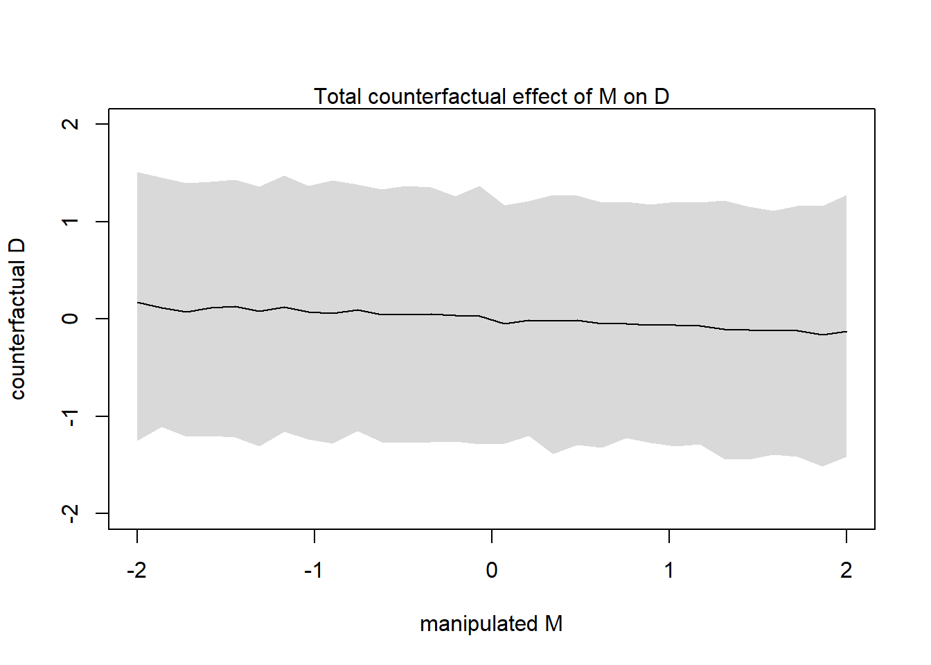
DAG Model 2

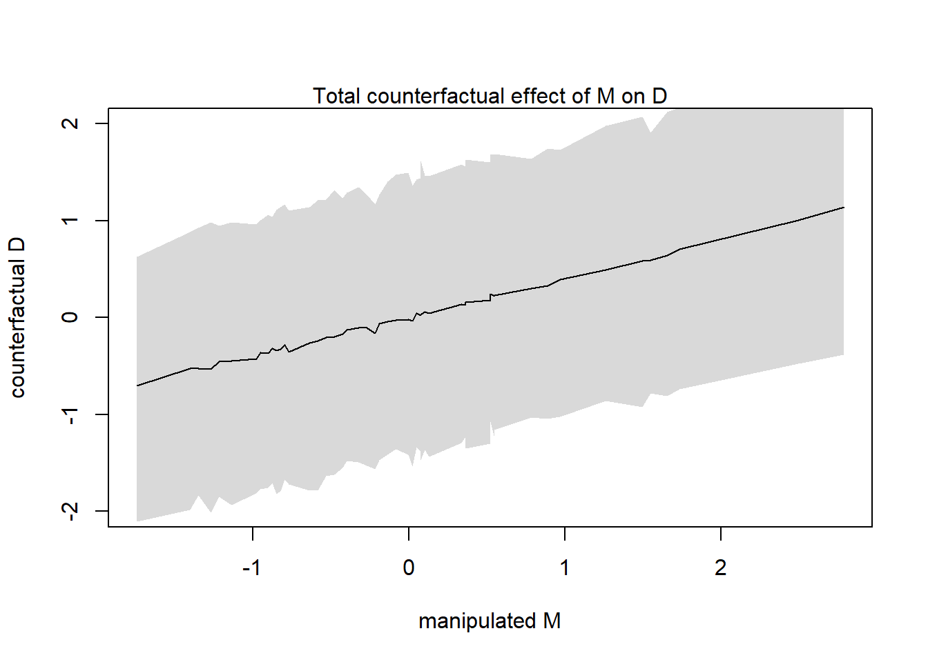
Let’s simulate a counterfactual for an average state with A=0 and the causal effect of manipulating M on D (note: manipulating M requires removing the arrows entering into M resulting in the DAG model 2):

M_seq <- seq(from=-2,to=2,length.out=30)

sim_dat <- data.frame(M=M_seq, A=0)

s <- sim(m5.3_A, data=sim_dat, vars="D")


{
plot(sim_dat$M, colMeans(s), ylim=c(-2,2), type="l",
     xlab="manipulated M", ylab="counterfactual D")
shade(apply(s,2,PI), sim_dat$M)
mtext("Total counterfactual effect of M on D")
}

It clear how the trend is less strong because there is no evidence for a strong influence of M on D.

Simulating counterfactual w/o `sim` function

Let’s simulate the counterfactual for manipulating A w/o using the sim function.

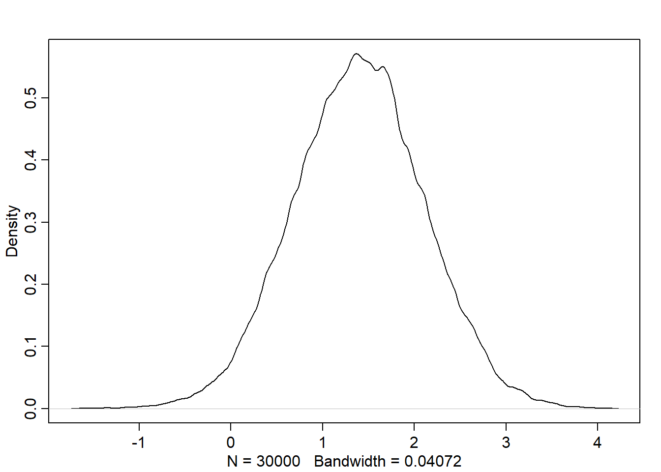
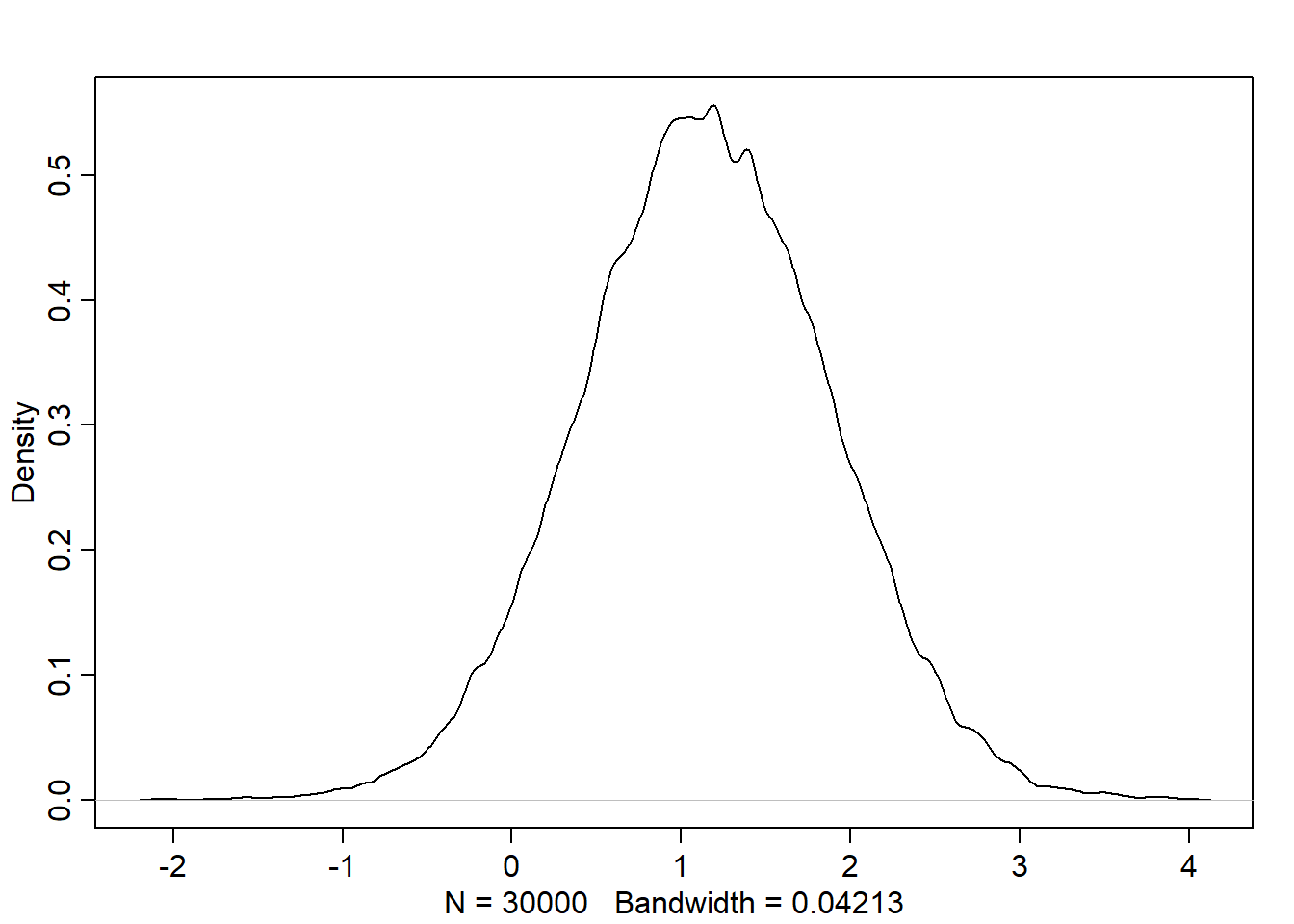
A_seq <- seq(from=-2, to=-2, length.out=30)
post <- extract.samples(m5.3_A)

# effect on M (distribution of M after simulating the counterfactual)
M_sim <- with(post, sapply(
  1:30,
  function(i) rnorm(1e3, aM + bAM*A_seq[i], sigma_M)
))

dens(M_sim)

# effect on D
D_sim <- with(post, sapply(
  1:30,
  function(i) rnorm(1e3, a + bA*A_seq[i] + bM*M_sim[i], sigma_M)
))

dens(D_sim)

Masked relationships

data("milk")
d <- milk
str(d)

'data.frame':   29 obs. of  8 variables:
 $ clade         : Factor w/ 4 levels "Ape","New World Monkey",..: 4 4 4 4 4 2 2 2 2 2 ...
 $ species       : Factor w/ 29 levels "A palliata","Alouatta seniculus",..: 11 8 9 10 16 2 1 6 28 27 ...
 $ kcal.per.g    : num  0.49 0.51 0.46 0.48 0.6 0.47 0.56 0.89 0.91 0.92 ...
 $ perc.fat      : num  16.6 19.3 14.1 14.9 27.3 ...
 $ perc.protein  : num  15.4 16.9 16.9 13.2 19.5 ...
 $ perc.lactose  : num  68 63.8 69 71.9 53.2 ...
 $ mass          : num  1.95 2.09 2.51 1.62 2.19 5.25 5.37 2.51 0.71 0.68 ...
 $ neocortex.perc: num  55.2 NA NA NA NA ...

Standardiaze the variables we want to use in the analysis

d$K <- standardize(d$kcal.per.g)
d$N <- standardize(d$neocortex.perc)
d$M <- standardize(d$mass)

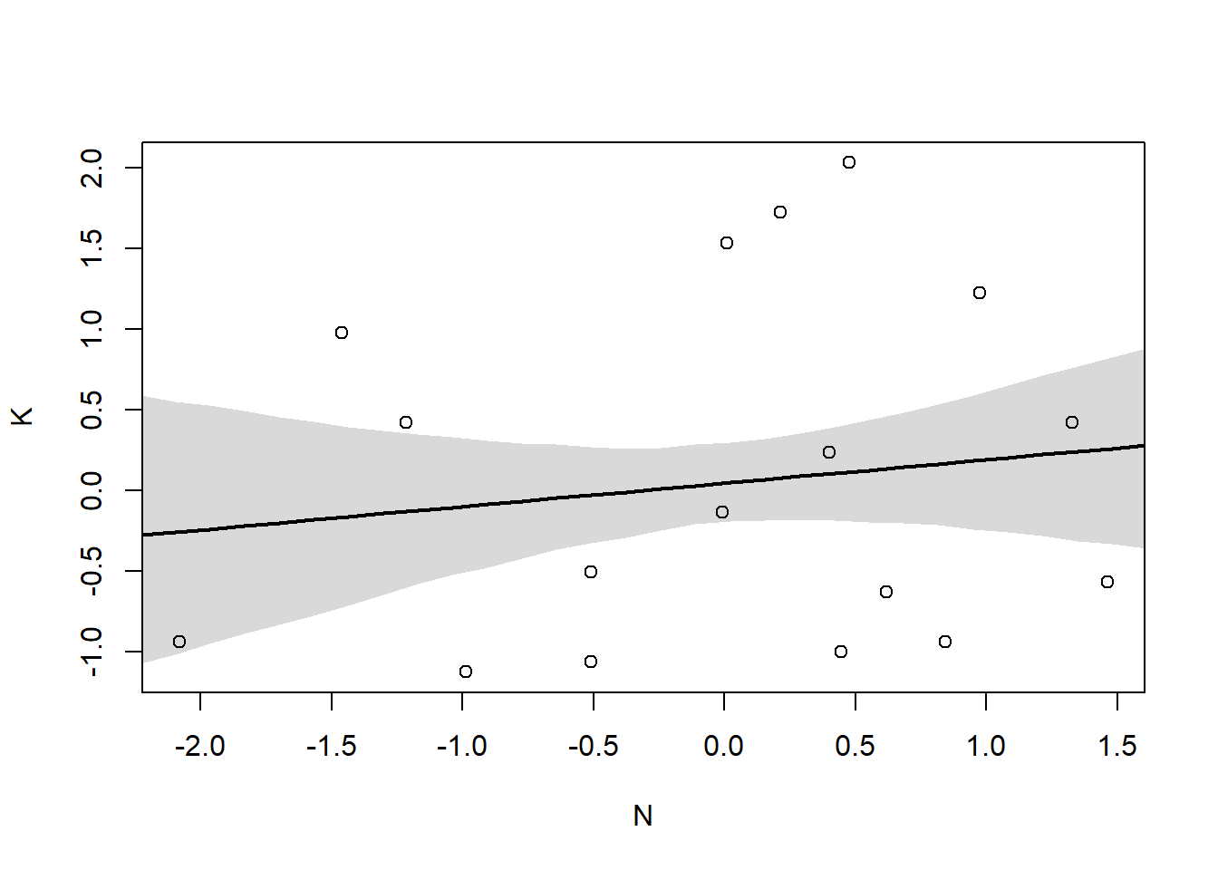
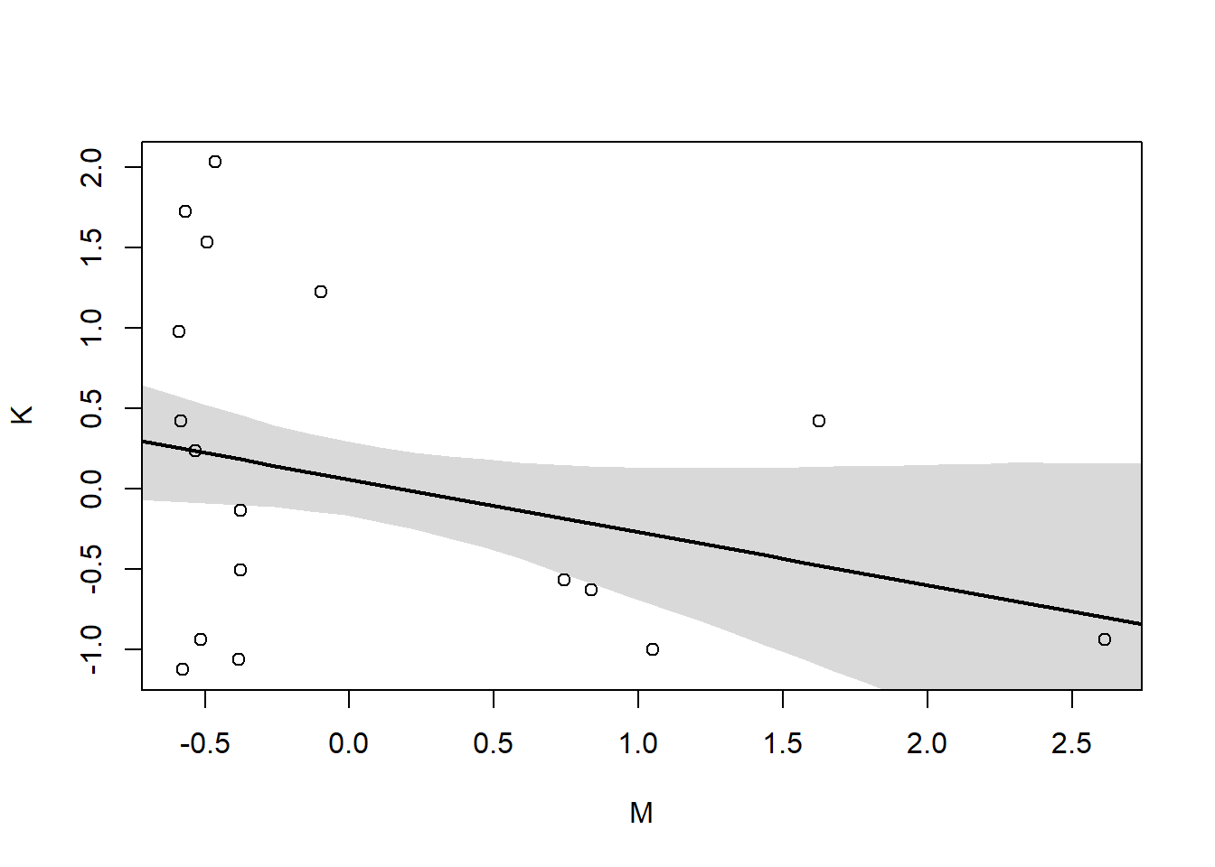
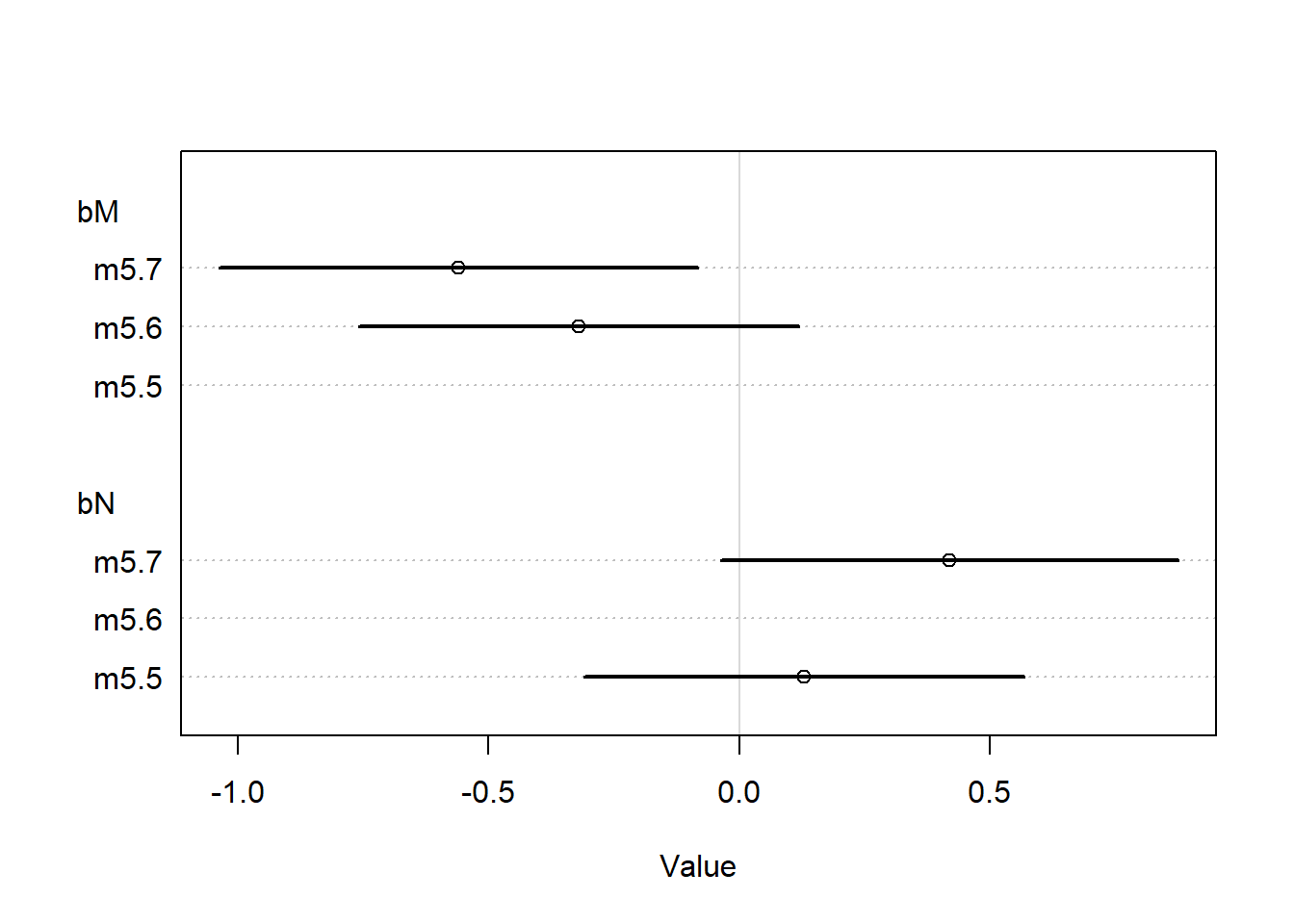
Model 1 (K ~ N): simple bivariate regression between K and N

\[ K_i \sim Normal(\mu_i, sigma) \] \[ \mu_i = \alpha + \beta_N N_i \] Define the model with vague priors

m5.5_draft <- quap(
  alist(
    K~dnorm(mu, sigma),
    mu <- a + bN * N,
    a~dnorm(0,1),
    bN~dnorm(0,1),
    sigma~dexp(1)
    
  ), data=d
)

Error in quap(alist(K ~ dnorm(mu, sigma), mu <- a + bN * N, a ~ dnorm(0, : initial value in 'vmmin' is not finite
The start values for the parameters were invalid. This could be caused by missing values (NA) in the data or by start values outside the parameter constraints. If there are no NA values in the data, try using explicit start values.

We want to conduct the analysis with complete cases only (i.e. cases shouldn’t have NA in the variables of interest)

# keep the rows that corresponds to complete cases for the variables we are interested in
dcc <- d[complete.cases(d$K, d$N, d$M),]

m5.5_draft <- quap(
  alist(
    K~dnorm(mu, sigma),
    mu <- a + bN * N,
    a~dnorm(0,1),
    bN~dnorm(0,1),
    sigma~dexp(1)
    
  ), data=dcc
)

Let’s simulate 50 priors:

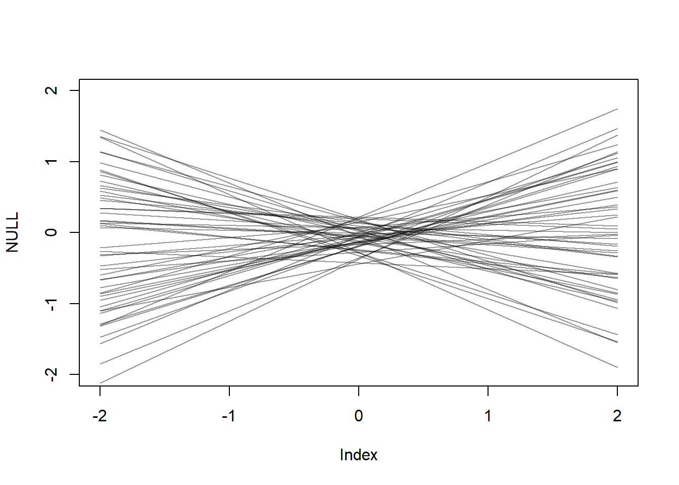
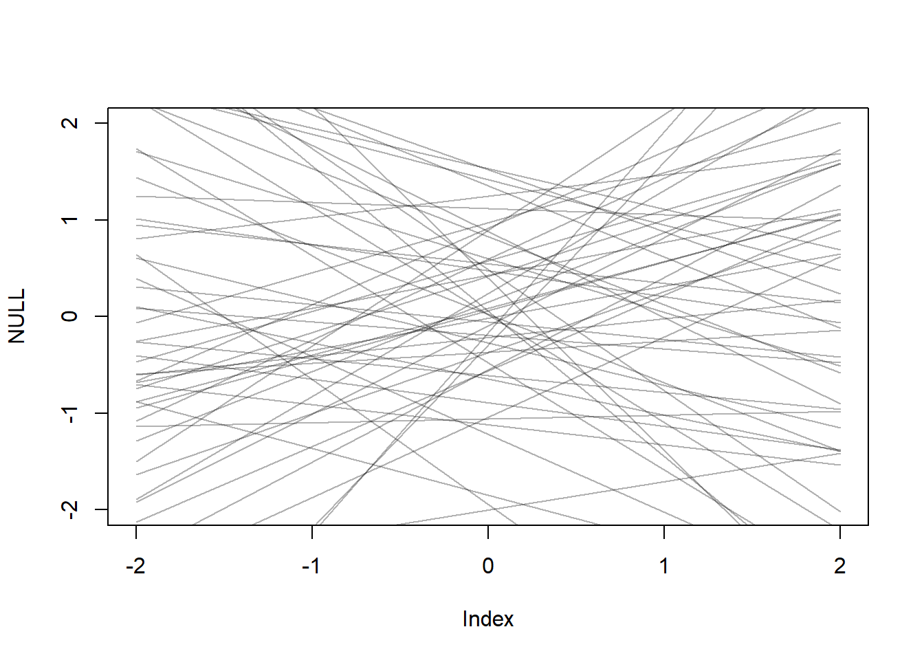
prior <- extract.prior(m5.5_draft)
xseq <- c(-2,2)
mu <- link(m5.5_draft, post=prior, data = list(N=xseq))

{
  plot(NULL, xlim=xseq, ylim=xseq)
  for (i in 1:50) lines(xseq, mu[i,], col=col.alpha("black", 0.3))
}

Let’s tighten the priors so that they stick closer and produce more reliable relationships:

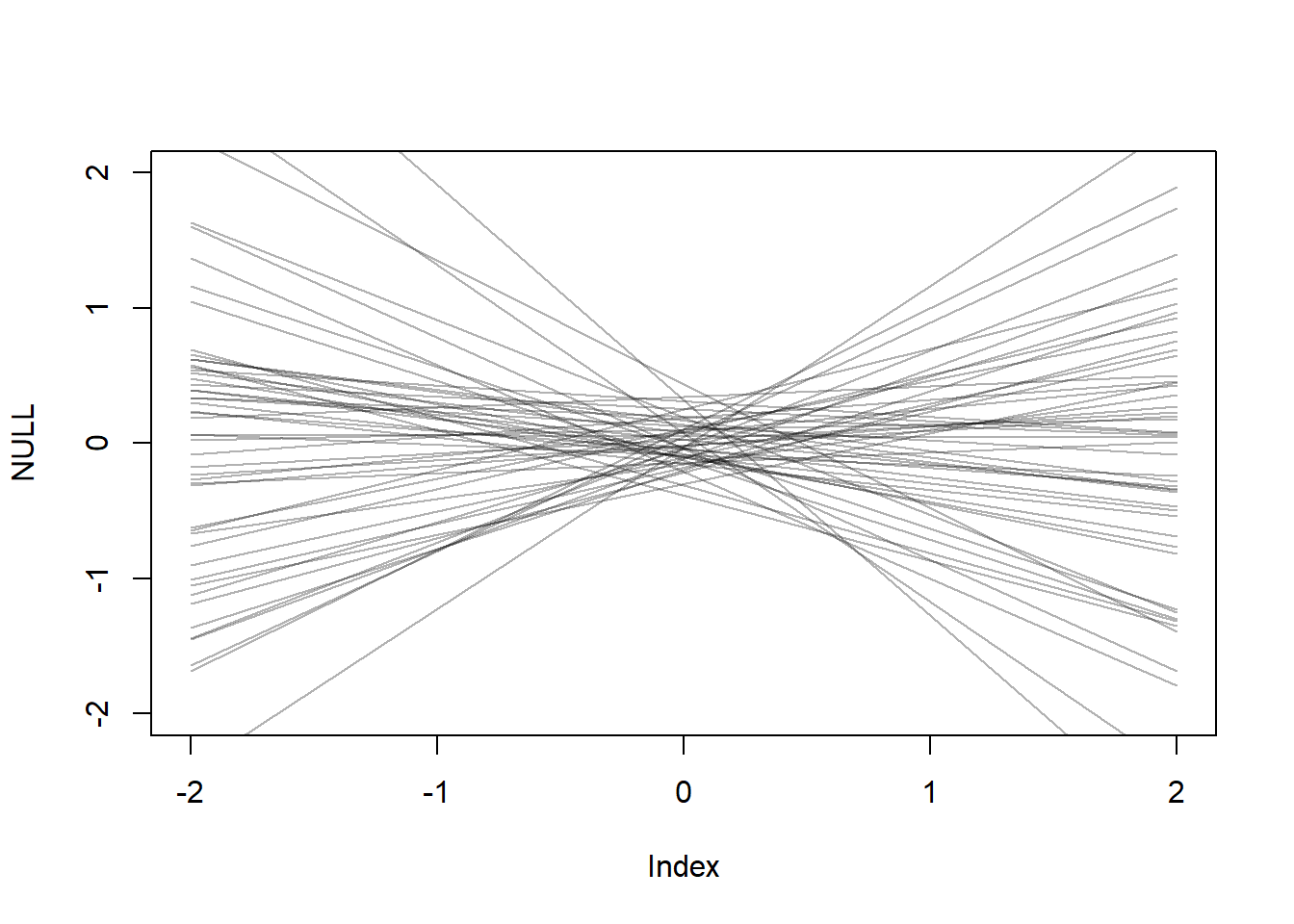
m5.5 <- quap(
  alist(
    K~dnorm(mu, sigma),
    mu <- a + bN * N,
    a~dnorm(0,0.2),
    bN~dnorm(0,0.5),
    sigma~dexp(1)
    
  ), data=dcc
)

prior <- extract.prior(m5.5)
xseq <- c(-2,2)
mu <- link(m5.5, post=prior, data = list(N=xseq))

{
  plot(NULL, xlim=xseq, ylim=xseq)
  for (i in 1:50) lines(xseq, mu[i,], col=col.alpha("black", 0.3))
}

xseq <- seq(from=min(dcc$N)-0.15, to=max(dcc$N)+0.15, length.out=30)
mu <- link(m5.5, data=list(N=xseq))
mu_mean <- apply(mu, 2, mean)
mu_PI <- apply(mu, 2, PI)
plot(K~N, data=dcc)
lines(xseq, mu_mean, lwd=2)
shade(mu_PI, xseq)

precis(m5.5)

            mean        sd       5.5%     94.5%
a     0.03990624 0.1544899 -0.2069984 0.2868109
bN    0.13324473 0.2237436 -0.2243407 0.4908302
sigma 0.99980248 0.1647006  0.7365791 1.2630259

N is slightly positivley associated with K.

Model 2 (K ~ M)

Remember that mass in the original dataset is the logarethem of mass (log-mass)

m5.6 <- quap(
  alist(
    K~dnorm(mu, sigma),
    mu <- a + bM * M,
    a~dnorm(0,0.2),
    bM~dnorm(0,0.5),
    sigma~dexp(1)
  ),
  data=dcc
)
precis(m5.6)

             mean        sd       5.5%      94.5%
a      0.05300796 0.1515525 -0.1892022 0.29521809
bM    -0.31900745 0.2238007 -0.6766842 0.03866927
sigma  0.94932747 0.1574741  0.6976535 1.20100142

Log-mass M is negatively associated with K.

xseq <- seq(from=min(dcc$M)-0.15, to=max(dcc$M)+0.15, length.out=30)
mu <- link(m5.6, data=list(M=xseq))
mu_mean <- apply(mu, 2, mean)
mu_PI <- apply(mu, 2, PI)
plot(K~M, data=dcc)
lines(xseq, mu_mean, lwd=2)
shade(mu_PI, xseq)

Model 1 and 2 aren’t useful in our case and they show no significant association

Model 3: Multivariate

\[ K_i \sim Normal(\mu_i, sigma) \]

\[ \mu_i = \alpha + \beta_N N_i + \beta_M M_i \]

m5.7 <- quap(
  alist(
    K~dnorm(mu, sigma),
    mu <- a + bN*N + bM * M,
    a~dnorm(0,0.2),
    bN~dnorm(0,0.5),
    bM~dnorm(0,0.5),
    sigma~dexp(1)
  ),
  data=dcc
)
precis(m5.7)

             mean        sd        5.5%      94.5%
a      0.06959672 0.1437680 -0.16017228  0.2993657
bN     0.42039090 0.2322482  0.04921335  0.7915685
bM    -0.56045516 0.2432229 -0.94917229 -0.1717380
sigma  0.84041552 0.1448683  0.60888805  1.0719430

plot(precis(m5.7))

Let’s compare with the previous models:

plot(coeftab(m5.5, m5.6, m5.7), pars=c("bM","bN"))

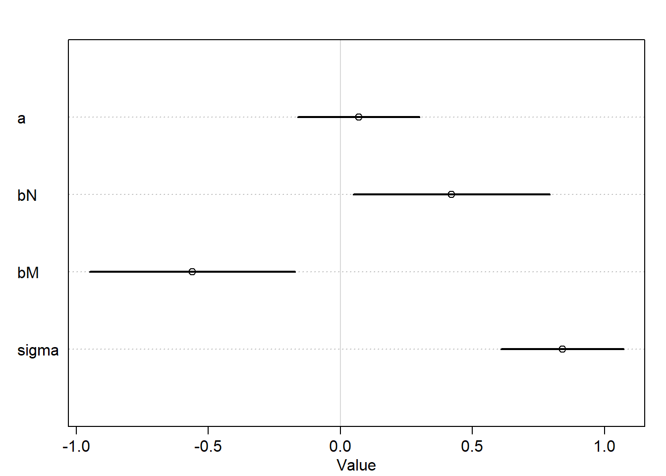
By incorporating both predictor variables in the regression, the posterior association of both with the outcome has increased. Also, the posterior means for N and M have both moved away from zero

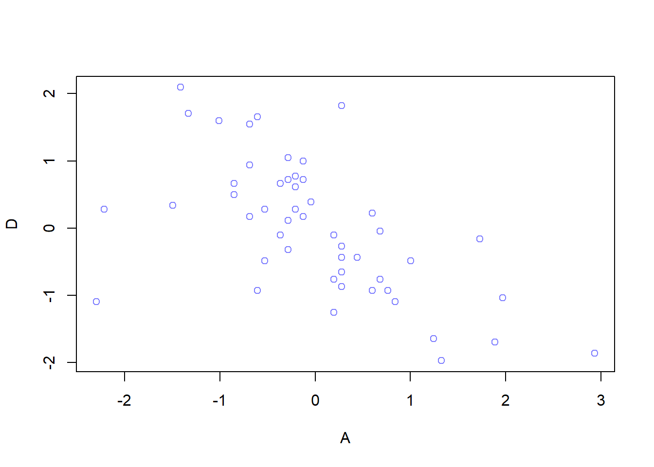
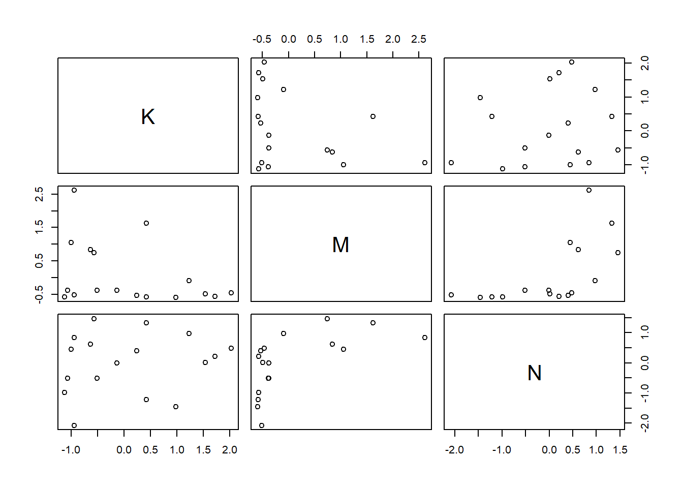
pairs(~K + M + N, dcc)

Categorical variables

Binary categories

library(rethinking)
data("Howell1")
d <- Howell1

Using the sex as a predictor for height, we have this model definition:

\(h_i \sim Normal(\mu_i, \sigma)\)

\(\mu_i = \alpha + \beta_m m_i\)

\(\alpha \sim Normal(178, 20)\)

\(\beta_m \sim Normal(0, 10)\)

\(\sigma \sim Uniform(0,50)\)

Where \(m_i\) is an indicator variable that takes the value 1 if the case is male, and zero otherwise.

This implies that the prior would have more uncertainty for male cases. See how thhe prior for male is wider:

mu_female <- rnorm(1e4, 178, 20)
mu_male <- rnorm(1e4, 178, 20) + rnorm(1e4, 0, 10)
precis(data.frame(mu_female, mu_male), hist=FALSE)

              mean       sd     5.5%    94.5%
mu_female 177.9726 20.09901 146.2121 210.2413
mu_male   177.8210 22.34856 141.8660 213.5161

This property for prior is not accepted in complex regression models.

Another way to encode categorical vars is using index variable, which is scalable to non-binary categories:

\(h_i \sim Normal(\mu_i, \sigma)\)

\(\mu_i = \alpha_{SEX[i]}\)

\(\alpha_j \sim Normal(178, 20) \space for \space j=1..2\)

\(\sigma \sim Uniform(0,50)\)

Now, look how the same prior is assigned to each category. However, we need to construct the index variable as follows:

# 2 if male
# 1 if female
d$sex <- ifelse(d$male==1,2,1)

m5.8 <- quap(
  alist(
    height ~ dnorm(mu, sigma),
    mu <- a[sex],
    a[sex] ~ dnorm(178,20),
    sigma ~ dunif(0,50)
  ),
  data=d
)

# depth=2 is needed to show any vector parameters
precis(m5.8, depth = 2)

           mean        sd      5.5%     94.5%
a[1]  134.91043 1.6069392 132.34223 137.47863
a[2]  142.57764 1.6974784 139.86474 145.29054
sigma  27.31006 0.8280497  25.98668  28.63344

We can find the expected difference between females and males as follows:

post <- extract.samples(m5.8)
post$diff_fm <- post$a[,1] - post$a[,2]
precis(post,depth = 2)

              mean        sd      5.5%      94.5%
sigma    27.286991 0.8253867  25.97253  28.619264
a[1]    134.932750 1.6115325 132.37565 137.531772
a[2]    142.558122 1.6988628 139.86985 145.285992
diff_fm  -7.625372 2.3367162 -11.34310  -3.897871
                                                                                                                       histogram
sigma                   <U+2581><U+2581><U+2581><U+2581><U+2583><U+2585><U+2587><U+2587><U+2583><U+2582><U+2581><U+2581><U+2581>
a[1]                    <U+2581><U+2581><U+2581><U+2581><U+2582><U+2585><U+2587><U+2587><U+2585><U+2582><U+2581><U+2581><U+2581>
a[2]    <U+2581><U+2581><U+2581><U+2581><U+2581><U+2583><U+2587><U+2587><U+2587><U+2583><U+2582><U+2581><U+2581><U+2581><U+2581>
diff_fm                                         <U+2581><U+2581><U+2581><U+2582><U+2587><U+2587><U+2583><U+2581><U+2581><U+2581>

This calculation is called a contrast.

Many categories

data(milk)

d <- milk

levels(d$clade)

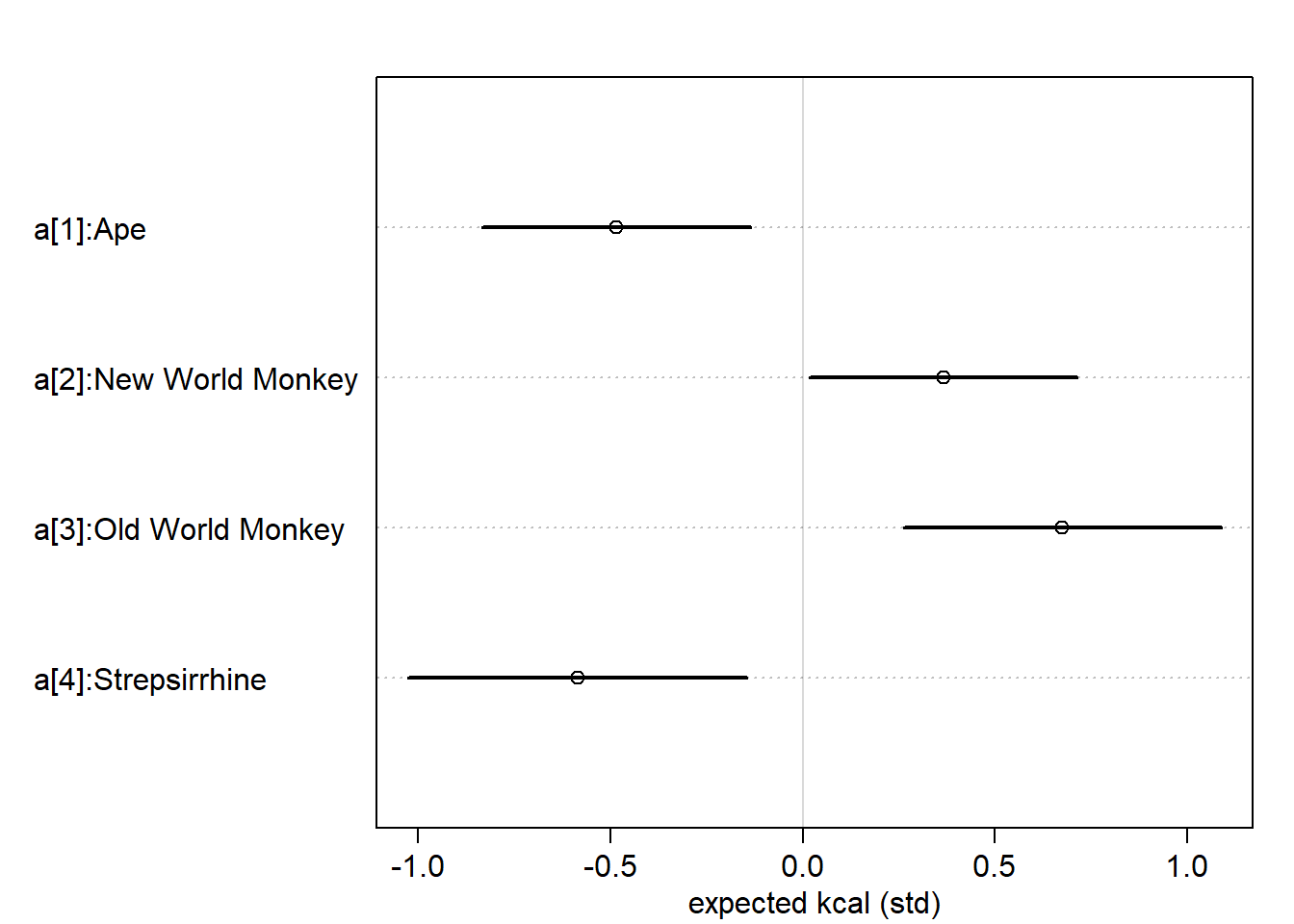
[1] "Ape"              "New World Monkey" "Old World Monkey" "Strepsirrhine"

d$clade_id <- as.integer(d$clade)

d$K <- standardize(d$kcal.per.g)
m5.9 <- quap(
  alist(
    K ~ dnorm(mu, sigma),
    mu <- a[clade_id],
    a[clade_id] ~ dnorm(0,0.5),
    sigma ~ dexp(1)
  ),
  data=d
)

labels <- paste("a[", 1:4, "]:",levels(d$clade), sep="")

plot(precis(m5.9, depth=2, pars = "a"), labels=labels, xlab="expected kcal (std)")

Exercises

Hard

1.In the divorce example, suppose the DAG is: M → A → D. What are the implied conditional independencies of the graph? Are the data consistent with it?

library(rethinking)
library(daggity)

Error in library(daggity): there is no package called 'daggity'

dag <- dagitty('dag{M -> A -> D}')

impliedConditionalIndependencies(dag)

D _||_ M | A

This is the same implied conditional independency that the data is consistent with as discussed in the chapter.

Assuming that the DAG for the divorce example is indeed M → A → D, fit a new model and use it to estimate the counterfactual effect of halving a State’s marriage rate M. Use the counterfactual example from the chapter (starting on page 140) as a template

Fit the new model

data("WaffleDivorce")

d <- list()
d$A <- standardize(WaffleDivorce$MedianAgeMarriage)
d$D <- standardize(WaffleDivorce$Divorce)
d$M <- standardize(WaffleDivorce$Marriage)

# M -> A -> D
mH2 <- quap(
  alist(
    # A -> D
    D ~ dnorm(mu, sigma),
    mu <- a + bA * A,
    a ~ dnorm(0,0.2),
    bA ~ dnorm(0, 0.5),
    sigma ~ dexp(1),
    
    # M -> A
    A ~ dnorm(mu_A, sigma_A),
    mu_A <- a_A + bM * M,
    a_A ~ dnorm(0,0.2),
    bM ~ dnorm(0, 0.5),
    sigma_A ~ dexp(1)
    
  ),
  data = d
)

Simulate the counterfactual effect of having a State’s marriage rate M

M_seq <- standardize(WaffleDivorce$Marriage * 0.5)
M_seq <- M_seq[order(M_seq)]

sim_dat <- data.frame(M=M_seq)

s <- sim(mH2, data=sim_dat, vars=c("A","D"))

{
  plot(sim_dat$M, colMeans(s$D), ylim=c(-2,2), type="l",
       xlab="manipulated M", ylab="counterfactual D")
  shade(apply(s$D,2,PI), sim_dat$M)
  mtext("Total counterfactual effect of M on D")
}

5. The Many Variablles and The Spurious Waffles

Model 1: D ~ A

Model 2: D ~ M

DAGs

Proposed DAG Model 1

Proposed DAG Model 2

Model 3: Multiple Regression

Simulating spurious association

Plotting multivariate posterior

1. Predictor residual

2. Posterior prediction plots

3. Counterfactual plots

DAG Model 1

DAG Model 2

Simulating counterfactual w/o sim function

Masked relationships

Model 1 (K ~ N): simple bivariate regression between K and N

Model 2 (K ~ M)

Model 3: Multivariate

Categorical variables

Binary categories

Many categories

Exercises

Hard

Simulating counterfactual w/o `sim` function