Lectures

Lecture 4: Categories & Curves

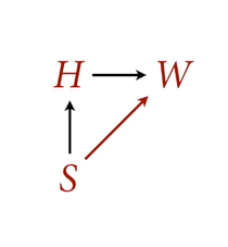
Let’s make a function that represents the relationships in this scientific (causal) model:

# simulation function #
sim_HW <- function(S,b,a) {
# S=1 female; S=2 male
  N <- length(S)
  # arbirtary parameters based on sex
  H <- ifelse(S==1, 150, 160) + rnorm(N, 0, 5)
  
  # a is the intercept; b is the slope
  W <- a[S] + b[S] * H + rnorm(N, 0, 5)
  data.frame(S, H, W)
}

# test the simulation function #

rbern <- function(n, p = 0.5) {
  rbinom(n, size = 1, prob = p)
}

# generate sexes for persons
S <- rbern(100) + 1
# pass the parameters a and b for each sex
dat <- sim_HW(S, b=c(0.5,0.6), a=c(0,0))
head(dat)

  S        H         W
1 1 149.8310  62.27643
2 1 146.0825  76.61531
3 2 159.5063  98.03304
4 2 153.9408  90.19251
5 1 142.7231  76.50352
6 2 162.7157 101.02463

Finding the causal effect involves conditioning on the confounder or mediator to block the association. This implies computing the difference between posterior prediction which is formally called computing the contrast.

Finding the total causal effect

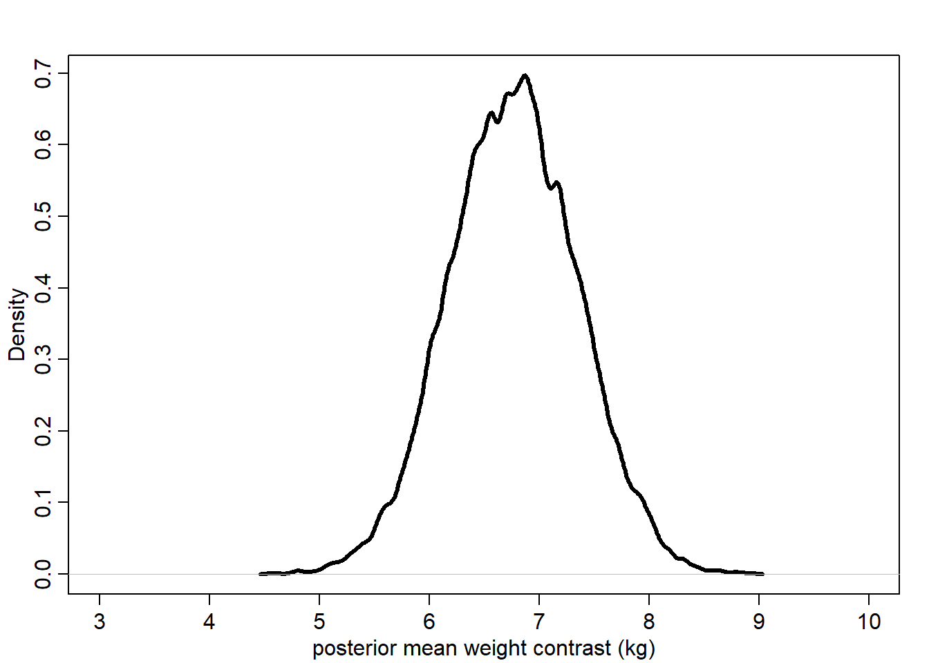
What’s the total causal effect of sex (through the two passes)? It is the difference made intervening. Let’s find that by testing

# female sample
S <- rep(1,100)
simF <- sim_HW(S,b=c(0.5,0.6),a=c(0,0))

# female sample
S <- rep(2,100)
simM <- sim_HW(S,b=c(0.5,0.6),a=c(0,0))

# effect of sex (male-female)
mean(simM$W - simF$W)

[1] 20.58828

Now, we want to define the statistical model (i.e. generative model) of weight:

\[ W_i \sim Normal(\mu_i, \sigma) \]

\[ \mu_i = \alpha_{S[i]} \]

\[ \alpha_j \sim Normal(60,10) \]

\[ \sigma \sim Uniform(0,10) \]

Let’s run the estimating model and synthetic sample

# observe sample (100 individuals)
S <- rbern(100)+1
dat <- sim_HW(S, b=c(.5,.6), a=c(0,0))

library(rethinking)

Loading required package: cmdstanr

This is cmdstanr version 0.7.1

- CmdStanR documentation and vignettes: mc-stan.org/cmdstanr

- CmdStan path: C:/Users/H/Documents/.cmdstan/cmdstan-2.34.1

- CmdStan version: 2.34.1

Loading required package: posterior

This is posterior version 1.5.0

Attaching package: 'posterior'

The following objects are masked from 'package:stats':

    mad, sd, var

The following objects are masked from 'package:base':

    %in%, match

Loading required package: parallel

rethinking (Version 2.40)

Attaching package: 'rethinking'

The following object is masked _by_ '.GlobalEnv':

    rbern

The following object is masked from 'package:stats':

    rstudent

# estimate posterior
m_SW <- quap(
  alist(
    W ~ dnorm(mu, sigma),
    mu <- a[S],
    a[S] ~ dnorm(60,10),
    sigma ~ dunif(0,10)
  ),
  data=dat
)

precis(m_SW, depth = 2)

           mean        sd      5.5%     94.5%
a[1]  74.145439 0.6641629 73.083979 75.206900
a[2]  94.912007 0.7492726 93.714525 96.109490
sigma  4.980696 0.3524650  4.417389  5.544004

Note that a is the average weight in the observed sample, stratified by sex.

Fit the model to the real data

library(rethinking)
data("Howell1")
d <- Howell1
d <- d[d$age >= 18, ]

dat <- list(
  W = d$weight,
  S = d$male + 1
)

m_SW <- quap(
  alist(
    W ~ dnorm(mu, sigma),
    mu <- a[S],
    a[S] ~ dnorm(60,10),
    sigma ~ dunif(0,10)
  ),
  data=dat
)

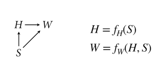
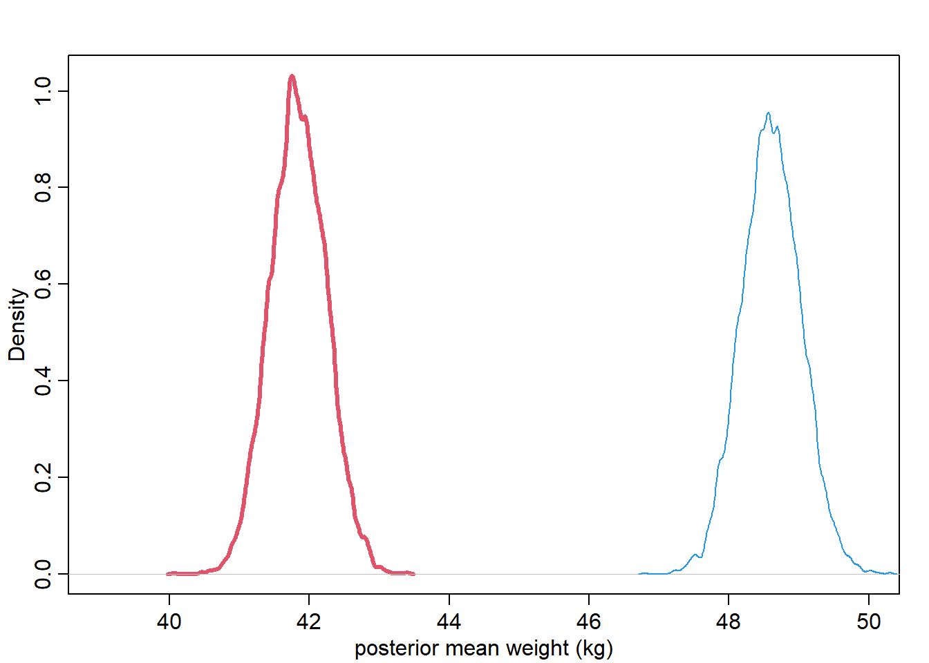
Find the mean weight for each sex (mean weight, NOT predicted weight!)

# sample from posterior (i.e. sample parameter values)
post <- extract.samples(m_SW)

# plot the posterior mean weight for each sex
{
  # female in red
  dens(post$a[, 1], xlim=c(39,50), lwd=3, col=2, xlab="posterior mean weight (kg)")
  dens(post$a[, 2], add=TRUE, col=4)
}

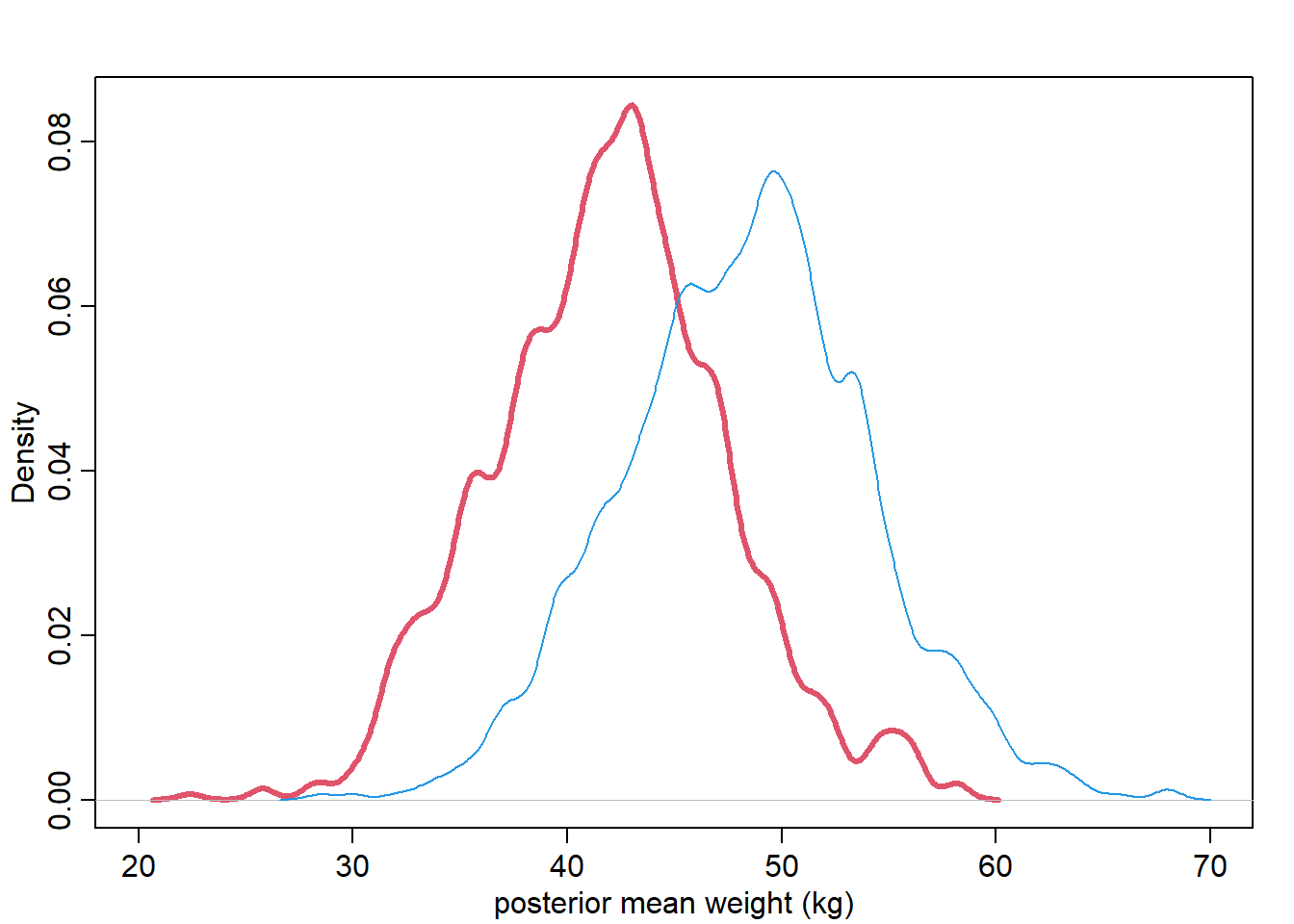
W1 <- rnorm(1e3, post$a[,1], post$sigma)
W2 <- rnorm(1e3, post$a[,2], post$sigma)


# plot the posterior predicted weight for each sex
{
  # female in red
  dens(W1, xlim=c(20,70), lwd=3, col=2, xlab="posterior mean weight (kg)")
  dens(W2, add=TRUE, col=4)
}

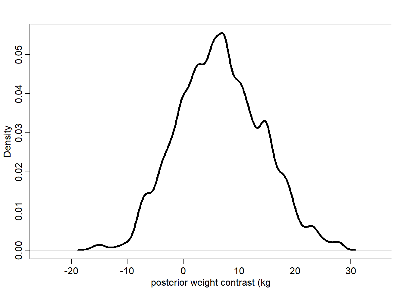
Compute contrast

To find the difference between posteriors of each category, we need to compute the contrast.

Note: overlap of distributions doesn’t indicate that they are the same or different!

1. Causal contrast in means

mu_contrast <- post$a[,2] - post$a[,1]

dens(mu_contrast, xlim=c(3,10), lwd=3, col=1, xlab="posterior mean weight contrast (kg)")

2. Weight contrast

We want to find the contrast in the distributions of individual people not averages

# simulate
W1 <- rnorm(1e3, post$a[,1], post$sigma)
W2 <- rnorm(1e3, post$a[,2], post$sigma)

# contrast
W_contrast <- W2 - W1
dens(W_contrast, xlim=c(-25,35), lwd=3, col=1, xlab="posterior weight contrast (kg")

Since we subtracted the posterior of women weights from the posterior of men weights, we can get the proportion at which the men have weight more than women by doing the following:

sum(W_contrast > 0) / 1e3

[1] 0.803

So 79% of the time, men are heavier than women in this population

sum(W_contrast < 0) / 1e3

[1] 0.197

So 20% of the time, women are heavier than women in this population

Direct causal effect of S on W

We need to block association through H = This means stratify by H.

The model is defined by:

\[ W_i \sim Normal(\mu_i, \sigma) \]

\[ \mu_i = \alpha_{S[i]} + \beta_{S[i]}(H_i - \bar{H}) \]

Note: it is a common practice to subtract predictor (i.e. H) from its average in order to make the intercept reflecting the outcome value when the predictor equals the average value. This is called “centering”.

The parameter now is a linear model. Let’s define the whole model with code:

data("Howell1")
d <- Howell1
d <- d[d$age >= 18, ]

dat <- list(
  W = d$weight,
  H = d$height,
  Hbar = mean(d$height),
  S = d$male+1
)

m_SHW <- quap(
  alist(
    W ~ dnorm(mu, sigma),
    mu <- a[S] + b[S] * (H - Hbar),
    a[S] ~ dnorm(60,10),
    b[S] ~ dunif(0,1),
    sigma ~ dunif(0,10)
  ),
  data=dat
)

Error in quap(alist(W ~ dnorm(mu, sigma), mu <- a[S] + b[S] * (H - Hbar), : non-finite finite-difference value [3]
Start values for parameters may be too far from MAP.
Try better priors or use explicit start values.
If you sampled random start values, just trying again may work.
Start values used in this attempt:
a = c(67.3159817200256, 64.0591387473614)
b = c(0.0486216379795223, 0.888933669775724)
sigma = 3.84191120741889